How to Freeze Excel 2010 Top and Bottom Rows

If you have a very large worksheet containing rows and rows of data it would be a lot easier for you if you were able to freeze both the top and bottom rows of your worksheet.

Unfortunately, there is no way to do this in MS Excel. You might think you could freeze your rows and split your worksheet window so that you can see your totals below the split, but again, unfortunately, Excel will not allow you to do this.

What a lot of Excel users do is put their column totals at the top of their columns instead of at the bottom. Yes, at first blush this may sound a bit awkward but if you think about it, it really has an added benefit, which is allowing you to easily add new rows to your data table.

Your top of the column totals could be added using either the SUM formulas the same as you would with your totals at the bottom, or you could leave the totals at the bottom of the columns and just add a referential formula in a row at the top of your columns.

There is another method that I just recently learned of and will now share with you.

Follow the steps below:

1. Open the workbook that contains the worksheet you would like to work on.
2. Click the View tab of your Ribbon.
3. In the Window group, click New to create a new window on the data in the worksheet you are using.
4. In the Window group, click the Arrange All tool to open the dialog box.
5. Be certain the Horizontal radio button is selected.

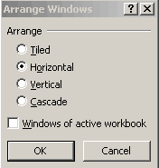
6. Click OK.

You should now see your two windows – one in the top half and the other in the lower half. Use your mouse to adjust the vertical height of both your windows. Be certain that your bottom window is large enough to hold your totals and the top window can fill the rest of the space.

You can now display your totals row(s) in your bottom window and freeze your top rows in the top window. Voila! You can now see all that you want/need to see!

Caveat: The only problem with this method is that your windows are not horizontally linked, which means that if you scroll one of your windows to the left or right, the other window does not scroll simultaneously.